K-means is a clustering algorithm that is relatively old yet it still in use today because of its simplicity and power.
Introduction
Unlike supervised learning algorithm, in unsupervised learning algorithms there is no notion of a label. We are simply given a set of input data and we want to conclude something from it. One idea is clustering. In this post we will focus on K-means algorithm.
In layman terms, clustering is grouping a collection of unlabeled data into similar sets. The resulting clusters will be vastly affected by how you decide if two points are similar to each other. Perhaps the simplest and most obvious measure of similarity is proximity where close by data points should belong to the same cluster.
K-means applies this idea in an iterative way, it starts with a random set of k-points $m_1, m_2, …, m_k$ that act as the centroid of the $k$ clusters to be determined (hence the name k-means) and it proceeds in two steps:
Assignment step: each point in the data set is assigned to the closest cluster based on the Euclidean distance to the cluster centroid. Mathematically speaking, the point $x$ is assigned to the cluster $C_i$ so that each cluster has a set of points $S_i$ such that $\lvert\lvert {x – m_i} \rvert\rvert \leq \lvert\lvert x – m_j \rvert\rvert \enspace \forall \enspace 1 \leq j \leq k$
Update step: recalculate the cluster centroid based on the new assigned points $m_i=\frac{1}{\rvert S_i \lvert}\sum \limits_{x_j \in S_i} x_j$
The algorithm keeps iterating until no more changes happen in data point assignment and centroid locations.
Worked Example
Suppose we are given the following dataset in $R_2$ and we want to cluster the data into k=2 clusters.
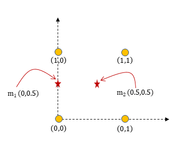
The first step is to pick 2 random initial locations for the cluster centroids. Let $m_1 = (0, 0.5)$ and $m_2 = (0.5, 0.5)$.
Iteration 1:
Assignment step:
| Distance to Centroid | $m1 (0, 0.5)$ | $m2 (0.5, 0.5)$ |
|---|---|---|
| $P1 (0, 0)$ | $\sqrt{(0-0)^2+(0-0.5)^2}=$ $0.5$ | $\sqrt{(0-0.5)^2+(0-0.5)^2}=0.707$ |
| $P2 (1,0)$ | $\sqrt{(1-0)^2+(0-0.5)^2}=1.118$ | $\sqrt{(1-0.5)^2+(0-0.5)^2}=$ $0.707$ |
| $P3 (0, 1)$ | $\sqrt{(0-0)^2+(1-0.5)^2}=$ $0.5$ | $\sqrt{(0-0.5)^2+(1-0.5)^2}=0.707$ |
| $P4 (1,1)$ | $\sqrt{(1-0)^2+(1-0.5)^2}=1.118$ | $\sqrt{(1-0.5)^2+(1-0.5)^2}=$ $0.707$ |
So P1 and P3 will be assigned to centroid $m1 (0, 0.5)$ while P2 and P4 will be assigned to centroid $m2 (0.5,0.5)$
Update step:
$$ \begin{aligned} m_1 &= \frac{1}{2} [(0,0)+(0,1)]=(0,0.5) \newline m_2 &= \frac{1}{2} [(1,0)+(1,1)]=(1,0.5) \end{aligned} $$
we can visualize the centroids ater the first iteration.
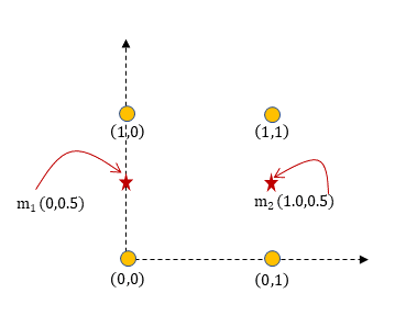
Iteration 2:
Assignment step:
| Distance to Centroid | $m1 (0, 0.5)$ | $m2 (0.5, 0.5)$ |
|---|---|---|
| $P1 (0, 0)$ | $\sqrt{(0-0)^2+(0-0.5)^2}=$ $0.5$ | $\sqrt{(0-1.0)^2+(0-0.5)^2}=1.118$ |
| $P2 (1,0)$ | $\sqrt{(1-0)^2+(0-0.5)^2}=1.118$ | $\sqrt{(1-1.0)^2+(0-0.5)^2}=$ $0.5$ |
| $P3 (0, 1)$ | $\sqrt{(0-0)^2+(1-0.5)^2}=$ $0.5$ | $\sqrt{(0-1.0)^2+(1-0.5)^2}=1.118$ |
| $P4 (1,1)$ | $\sqrt{(1-0)^2+(1-0.5)^2}=1.118$ | $\sqrt{(1-1.0)^2+(1-0.5)^2 }=$ $0.5$ |
And no new change in assignment will be done and the algorithm terminates.
Python Implementation
We can easily implement the above two steps in a couple of lines of python.
def kMeans(X, k):
    m = np.random.permutation(X)[:k]
    changes = True
    clusters = np.zeros(X.shape[0])
    while changes:
        changes = False
        for i in range(len(X)):
            idx = np.argmin(dist(X[i,:], m))
            if idx != clusters[i]:
                changes = True
            clusters[i] = idx

        for j in range(len(m)):
            m[j,:] = np.sum(X[clusters == j,:],axis=0)/np.sum(clusters == j)

    return m, clusters
And here is the definition of function dist
def dist(x, y):
    return np.sqrt(np.sum((x - y) ** 2, axis=1))
Picking K
At this point you might be asking the questions how to pick the correct number of clusters because the choice of k can generate completely different result. A good technique is to use the elbow method .
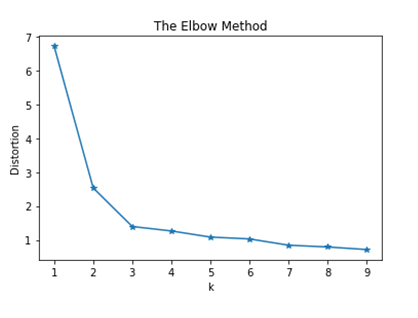
The elbow method is one of the most popular methods to determine the optimal number of clusters. We plot for different value of K on the x-axis, the distortion on the y-axis. We define distortion as the sum of distance between the data point and the centroid. Distortion = $\sum \lvert \lvert x_i-m_c \rvert \rvert $. At certain value of K we will notice shift in the graph trend which determines the optimal value of K.
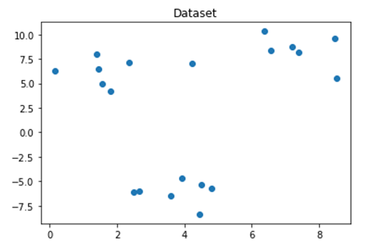
Let’s start by some arbitrary dataset consisting of three clusters as shown in the next figure, of course in real life we do not know in advance the actual number of clusters but we will use this example to see how the elbow method will do relative to what we know to be true.
from sklearn.datasets import make_blobs
x, y = make_blobs(n_samples=20, centers=3, n_features=2)
plt.plot()
plt.title('Dataset')
plt.scatter(x[:,0], x[:,1])
plt.show()
The next step is to apply k-means clustering algorithm for a range of value, calculate the distortion and plot it as a function of K. In this example we will try the k values in the range 1 to 10.
distortions = []
K = range(1,10)
for k in K:
    m, c = kMeans(x, k)
    distortion = 0
    for i in range(len(x)):
            distortion = distortion + np.min(dist(x[i,:], m))
    distortions.append(distortion/ x.shape[0])
We can then plot the distortions as a function of k. we then notice the elbow shape the curve makes at K=3 indicating the optimal value for the number of clusters.
plt.plot(K, distortions, '*-')
plt.xlabel('k')
plt.ylabel('Distortion')
plt.title('The Elbow Method')
plt.show()
Shortcomings
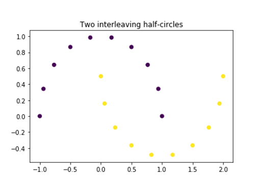
Because we are using the Euclidean distance when measuring the distance to the centroids, K-means algorithm prefer clusters that have circular shapes even when a better cluster shape is more appropriate. For example, let’s look at dataset of two interleaving circles (make_moons in sklearn).
from sklearn.datasets import make_moons
x, y = make_moons(n_samples=20)
plt.plot()
plt.title('Two interleaving half-circles')
plt.scatter(x[:,0], x[:,1],c=y)
plt.show()
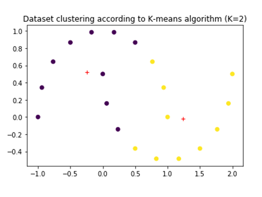
However, if we try to apply K-means algorithm using two clustering we will get two different clusters. Although it is a valid clustering it might not be the best way to divide the dataset to make inferences about the dataset.
Matrix Factorization Perspective
I learnt about this idea from the fantastic book Machine Learning Refined book. The books is filled with many insights about machine learning algorithms from an optimization point of you and I encourage you to check it out.
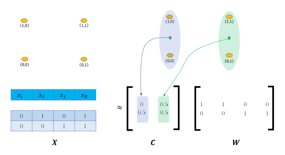
In our implementation, there are a set of points $X$ and the aim is to find K cluster centroids $C$ and assign each point $x$ to a particular cluster $c_k$ so that the assigned centroid is as close to the point as possible. i.e., if $e_k$ is all zeros vector except at entry k, then we want:
$$ C e_k = c_k \approx x_p \quad \text{for all points} \quad x_p \in X $$
The trick is we can rewrite this objective in matrix notation as $CW \approx X$, and lo and behold we arrive at the canonical matrix factorization from. In this from, $W$ is the weight matrix with the special constraint that each column contains a single nonzero entry that determines assignment of points to clusters. The next figure shows this framing for our worked example.
In this framing, K-means can be analyzed as an optimization problem with an objective function to be minimized and we can track and analyze the progress of the algorithm on each iteration.
Conclusion
In this post, we looked at the K-means clustering algorithm. We then looked at the algorithm steps and visualized some examples. We also discussed how to determine the optimal number of clusters and when the algorithm might not produce the best results. Finally, we discussed how K-means, a heuristic algorithm, can be viewed from the lens of an optimization framework.