The Root Mean Square Error (RMSE) is a common loss function used in machine learning for regression tasks that measures the average distance between the predicted and true values. However, what implicit modeling assumptions are me making when we use such error to evaluate the model fit?
Consider a dataset $(X, Y)$ containing $N$ instances and we want to train a regression model. Our goal is to make predictions for the target variable $y$ given some value of the input variable $x$. For any ML model to work there have to be some relationship between the input variable $x$ and the output variable to be able to write the output as a function of the input ($y=f(x)$). For simplicity, we assume that this relationship is linear. Hence, our function has the form $f(x) = w_0 + w_1x_i$.
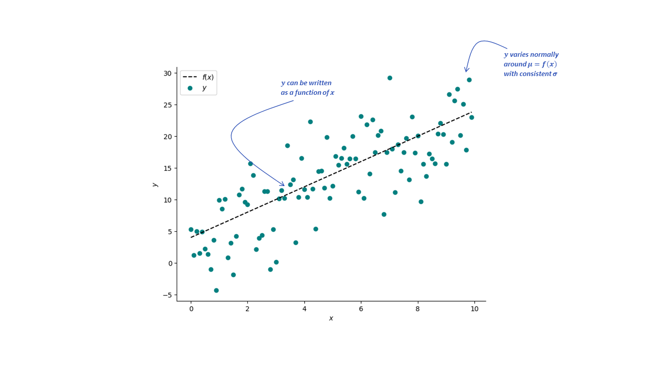
Consider the dataset in the plot below, there isa general linear trend but the target variables $y$ don’t fall perfectly on a straight line. To account for that, we update our model so that for each output we add a random noise component $\epsilon_i$. This noise component is random variable following a normal distribution with zero mean and variance $\sigma^2$.
Our model now takes the form:
$$ \begin{aligned} y_i &= f(x_i) + \epsilon_i \cr &= w_0 + w_1x_i + \epsilon_i \hspace{1em} \text{where}\hspace{1em} \epsilon_i \sim \mathcal{N}(0, \sigma^2) \end{aligned} $$
which consists of two components:
- A deterministic component $w_0 + w_1x_i$
- A random component $\epsilon_i$
Our goal by training the model is to find the optimal values of $w_0$ and $w_1$. Because the target variable is the sum of a deterministic component and a Gaussian random variable, it also a Gaussian random variable:
$$ \begin{aligned} P(y_i|x_i, w_0, w_1,\sigma^2) &\sim w_0 + w_1x_i + \mathcal{N}(0, \sigma^2) \cr &\sim \mathcal{N}(\mu=w_0 + w_1x_i, \sigma^2) \end{aligned} $$
The density $P(y_i|x_i, w_0, w_1,\sigma^2)$ is the likelihood of the ith data point. Because we have $N$ data points we are interested in the joint density
$$ P(y_1,y_2,…,y_N|x_1,x_2,…,x_N, w_0, w_1,\sigma^2) $$
It is reasonable to assume that the noise at each data point is independent of the noise at other points. We can then factorize the joint density into $N$ independent terms:
$$ \begin{aligned} P(y_1,y_2,…,y_N|x_1,x_2,…,x_N, w_0, w_1,\sigma^2) \cr = \prod_{i=1}^N P(y_i,|x_i, w_0, w_1,\sigma^2) \cr = \mathcal{N}(\mu=w_0 + w_1x_i, \sigma^2) \end{aligned} $$
We want to find $w_0$ and $w_1$ that maximizes the likelihood. Since the log function is monotonic we will maximize the log likelihood instead
$$ \begin{aligned} \log L &= \sum_{i=1}^{N}\log(\frac{1}{\sqrt{2\pi\sigma^2}} e^{-\frac{1}{2\sigma^2}(y_i - w_0 - w_1x_i)^2)}\cr &= \sum_{i=1}^{N}{-\frac{1}{2}\log 2\pi - \log\sigma - \frac{1}{2\sigma^2}\sum_{i=1}^{N}(y_i - w_0 - w_1x_i)^2}\cr &= -\frac{N}{2}\log 2\pi - N\log\sigma - \frac{1}{2\sigma^2}\sum_{i=1}^{N}(y_i - w_0 - w_1x_i)^2 \end{aligned} $$
To maximize $\log L$ we need to minimize the third term:
$$ \frac{1}{2\sigma^2}\sum_{i=1}^{N}(y_i - (w_0 + w_1x_i))^2 $$
which is exactly the Mean Square Error between the target and predicted values.
These assumptions were summarized sufficiently in the Bayes Rules! Book; using the RMSE is equivalent to modeling the target variable $Y_i$ as
$$y_i \sim N(\mu_i, \sigma) \hspace{1cm} \text{with} \hspace{0.2cm} \mu_i = f(X_i)$$
with the following assumptions:
Structure of the relationship: The typical outcome $Y$ can be written as a function of $X$
Structure of the variability: At any $X$ value, $Y$ varies normally around $\mu$ with consistent $\sigma$
Structure of the data: Conditioned on $X$, the target variable $Y$ on case $i$ is independent of the target variable on any case $j$
Interesting, if we have a trivial model that always predicts the mean value it will have an RMSE equals to the standard deviation of the data.
$$ \text{RMSE} \begin{aligned} &= \sqrt{\sum_i (y_i - \bar{y})^2} \cr &= \sigma(Y) \end{aligned} $$
Given this observation, the mean value of the training data can be used as a baseline in regression tasks. Furthermore, we can define the quantity Fraction of the variance unexplained (FUV) that is the ratio of the MSE to the variance where it equals 1 for a trivial model and 0 for a perfect model.
$$ \begin{aligned} R^2 &= 1 - \text{FUV} \cr &= 1 - \frac{\Sigma(y_i - \bar{y})^2}{\text{var}(y)} \end{aligned} $$