The Naïve Bayes classifier is a popular machine learning algorithm. In this post we will discuss why it still works in practice even when the (naïve) conditional independence assumption is violated.
Introduction
The Naïve Bayes classifier is a machine algorithm that can be used for classification tasks, similar to the perceptron algorithm. It is a probabilistic machine learning method which means it relies on probability theory to calculate the probability of a specific class given the input features.
For example, consider an input instance $X=(x_1,x_2,…,x_n)$ and output labels $Y \in$ {$+1,-1$} , the Naïve Bayes classifier calculates $P(Y=+1│x_1,x_2,…,x_n)$ and $P(Y=-1│x_1,x_2,…,x_n)$ and then picks the class that has a higher probability. To calculate these probabilities, the algorithm relies on Bayes rule which allows the probability defined above to be rewritten. Let $C_k \in$ {$+1,-1$} then:
$$ P(Y=C_k│x_1,x_2,…,x_n ) = \frac{P(x_1,x_2,…,x_n│Y=C_k) P(Y=C_k)}{P(x_1,x_2,…,x_n)} $$
Now, the naïve conditional independence assumption comes into play. Basically the algorithm assumes that the features are conditionally independent on the output label $C_k$ and this allows us to rewrite the term $P(x_1,x_2,…,x_n│Y=C_k)$ as a product of easier to compute terms, mainly:
$$P(x_1,x_2,…,x_n│Y=C_k)=\prod \limits_{i=1}^{n} P(x_i│Y=C_k)$$
What is conditional independence?
Before we go further let’s take a detour and give some intuition on what it means to be conditionally independent. For starters, two events A and B are independent if the occurrence of one event has no effect on the occurrence of the other, in probability terms we say $P(A│B) = P(A)$ if $A$ and $B$ are independent. For example, the probability of the event $A$: a coin will land heads and the event $B$: it is raining outside are independent.
However, conditional independence is always with respect to a third event so we say events $A$ and $B$ are conditionally independent given event $C$, in probability terms we say $P(A│B,C)=P(A│C)$ if $A$ and $B$ are conditionally independent given $C$.
To understand it better let us consider this nice example. Suppose that we toss the same coin twice where event $A$ is the outcome of the first toss and event $B$ is the outcome of the second toss, both events are dependent on the bias of the coin (its tendency to produce a certain output more) Now if $C$ is the event that the coin is double sided then once we observe the event $C$ the output of event $B$ has no effect on the outcome of event $A$, hence, events $A$ and $B$ are conditionally independent given event $C$.
What Happens in practice?
In practice, the Naïve assumption is often violated. For example, trying to predict a plant type based on width, height and color of the leaves. The classifier assumes that all these features are independent without consideration of their effect on each other. In this case the width and height are dependent so the assumption is over estimating the true probability. Another example, in text classification, each classification class $C_k$ considers all possible text values for word $i$ regardless on other words within a small window of that word. As such, the conditional independence assumption will often either over estimate or underestimate the probability $P(x_1,x_2,…,x_n│Y=C_k)$ which makes the total probability $P(Y=C_k│X)$ incorrect. So where is the catch?
Why does it work?
The answer to this question appeared in a paper from 1997 titled On the Optimality of the Simple Bayesian Classifier under Zero-One Loss. In that paper, the authors argued that the although the Naïve Bayes algorithm only estimated the probabilities $P(Y=+1│X)$ and $P(Y=-1│X)$.
Let $r = P(Y=+1)\prod \limits_{i=1}^{n} P(x_i│Y=+1)$ and $s = P(Y=-1)\prod \limits_{i=1}^{n} P(x_i│Y=-1)$, the output of the classifier is optimal if and only if:
$$ (P(Y=+1│X)>1/2 \enspace\text{and}\enspace r \geq s) \enspace\text{or}\enspace (P(Y=+1│X)<1/2 \enspace\text{and}\enspace r \leq s) $$
In other words, it does not matter if the Naïve Bayes classifier overestimatea or under estimatea the probabilities as long as the correct ratio is maintained between the true and estimated probabilities.
To make this idea of optimality clearer, let’s us describe an example, that appeared in the same paper, about a dataset with three Boolean attributes $A$, $B$ and $C$ (each attribute can have only the values 0 or 1). Assume that $P(+) = P(-) = \frac{1}{2}$ i.e. negative and positive classes are equally probable in the dataset. Furthermore, assume that $A$ and $C$ are independent but $A = B$ which clearly violates the conditional independence assumption of Naïve Bayes.
A theoretical optimal classifier will choose to ignore the attribute $B$ because it does not add any new information and it will calculate the probabilities $P(Y=+1│X)$ and $P(Y=-1│X)$ as follows:
$$ \begin{aligned} P(Y=+1│X) &= \frac{P(A│Y=+1)P(C│Y=+1)P(Y=+1)}{P(X)} \newline \enspace \newline P(Y=-1│X) &= \frac{P(A│Y=-1)P(C│Y=-1)P(Y=-1)}{P(X)} \end{aligned} $$
As such, the optimal classifier will assign the positive $+$ class if $P(Y=+1│X)- P(Y=-1│X)>0$ using the above expression for expansion and simplifying the result yields:
$$ \begin{equation} \label{optimal decision} P(A│Y=+1)P(C│Y=+1)-P(A│Y=-1)P(C│Y=-1)>0 \end{equation} $$
On the other hand, the Naïve Bayes classifier does not ignore the attribute B and it is included in the calculations which give the following definitions for $P(Y=+1│X)$ and $P(Y=-1│X)$:
$$ \begin{aligned} P(Y=+1│X) &= \frac{P(A│Y=+1)P(B│Y=+1)P(C│Y=+1)P(Y=+1)}{P(X)} \newline \enspace \newline P(Y=-1│X) &= \frac{P(A│Y=-1)P(B│Y=-1)P(C│Y=+1)P(Y=-1)}{P(X)} \end{aligned} $$
The Naïve Bayes classifier assigns the positive $+$ class if $P(Y=+1│X)- P(Y=-1│X)>0$ using the above expression for expansion, the fact that $A = B$ and simplifying the result yields:
$$ \begin{equation} \label{naive decision} P(A│Y=+1)^2 P(C│Y=+1)-P(A│Y=-1)^2 P(C│Y=-1)>0 \end{equation} $$
We can simplify equations $\eqref{optimal decision}$ and $\eqref{naive decision}$ even more by applying the Bayes rule again where we can rewrite $P(A│Y=+1) = \frac{P(Y=+1│A)P(A)}{P(Y=+1)}$, $P(A│Y=-1)=\frac{P(Y=-1│A)P(A)}{P(Y=-1)}$ and we can also do the same for $P(C│Y=+1)$ and $P(C│Y=-1)$.
Plugging these rewrites into the optimal classifier decision equations it becomes:
$$\frac{P(Y=+1|A)P(A)}{P(Y=+1)}\frac{P(Y=+1|C)P(C)}{P(Y=+1)}-\frac{P(Y=-1|A)P(A)}{P(Y=-1)}\frac{P(Y=-1|C)P(C)}{P(Y=-1)}>0$$
Using the fact that $P(+) = P(-) = \frac{1}{2}$ we get:
$$P(Y=+1|A)P(A)P(Y=+1|C)P(C)-P(Y=-1│A)P(A)(Y=-1|C)P(C)>0$$
Cancelling $P(A)P(C)$ from both sides:
$$ \begin{equation} \label{optimal decision simplified} P(Y=+1│A)P(Y=+1│C)-P(Y=-1│A)(Y=-1│C)>0 \end{equation} $$
Similarly, plugging these rewrites into the Naïve Bayes classifier decision equations it becomes:
$$\left(\frac{P(Y=+1|A)P(A)}{P(Y=+1)}\right)^2\frac{P(Y=+1|C)P(C)}{P(Y=+1)}-\left(\frac{P(Y=-1│A)P(A)}{P(Y=-1)}\right)^2 \frac{P(Y=-1│C)P(C)}{P(Y=-1)}>0$$
Using the fact that $P(+) = P(-) =\frac{1}{2}$ we get:
$$P(Y=+1│A)^2 P(A)^2 P(Y=+1│C)P(C)-P(Y=-1│A)^2 P(A)^2 (Y=-1│C)P(C)>0$$
Cancelling $P(A)^2P(C)$ from both sides:
$$ \begin{equation} \label{naive decision simplified} P(Y=+1│A)^2 P(Y=+1│C)-P(Y=-1│A)^2 (Y=-1│C)>0 \end{equation} $$
Let $P(Y=+1│A)=p$ and $P(Y=+1│C)=q$ so $P(Y=-1│A)=1-p$ and $P(Y=-1│C)=1-q$. Plugging p, q into the decision functions \eqref{optimal decision simplified} and \eqref{naive decision simplified} (to make the expressions more readable) we obtain:
The optimal classifier decision:
$$ \begin{aligned} P(Y=+1|A)P(Y=+1|C)-P(Y=-1|A)(Y=-1|C) &> 0 \newline pq-(1-p)(1-q) &> 0 \newline pq-(1+pq-p-q) &> 0 \newline pq-1-pq+p+q &> 0 \newline -1+p+q &> 0 \newline \end{aligned} $$
Which results in a decision boundary descibed by:
$$ \begin{equation} \label{optimal final} q > 1-p \end{equation} $$
The Naïve Bayes classifier decision:
$$
\begin{aligned}
P(Y=+1│A)^2 P(Y=+1│C)-P(Y=-1│A)^2 (Y=-1│C) &> 0 \newline
p^2 q-(1-p)^2 (1-q) &> 0 \newline
p^2 q-(1-p)^2+q(1-p^2 ) &> 0 \newline
q(p^2+(1-p)^2 )-(1-p^2 ) &> 0
\end{aligned}
$$
Which results in a decision boundary descibed by:
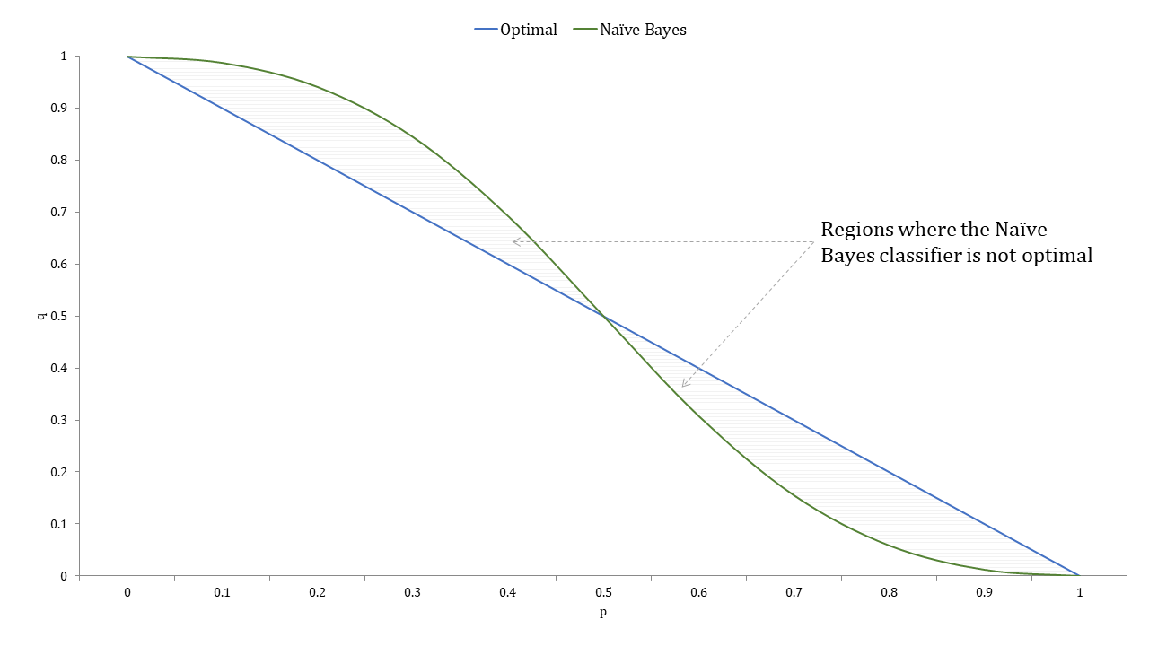
$$ \begin{equation} \label{naive final} q > \frac{(1-p)^2}{p^2+(1-p)^2} \end{equation} $$
The figure below shows the plot of these two decision boundaries \eqref{optimal final} and \eqref{naive final}. Notice that the two decision boundary are exactly equally at only three points the Naïve Bayes classifier is optimal except only in the two shaded regions that are above one of the curves and below the other where it disagrees with the optimal procedure. As such, the Naïve Bayes classifier is optimal in a far larger region than just wanting the probabilities to be exact which makes it much more successful in practice.
Conclusion
In this post, we looked at the Naïve Bayes algorithm. We then looked at the conditional independence assumption and examples of when it is violated in practive. We then looked at why Naïve Bayes works so well in practice.