The perceptron is a learning algorithm. A rather simple one yet surprising, it can acheive very good results as we will explore in this post.
Introduction
The perceptron is used for classification task where there are two categories and the objective is to learn how to differentiate between them. For example, whether an email is spam? Or whether a house will sell over a certain asking price?
Traditionally, for each object we want to classify a number of features are collected that best describe the object. In the house example mentioned earlier, the features might be the number of rooms, total area, number of bathrooms, etc. As a result we end up with a number of numerical features describing each object (instance) (Note: categorical features can be converted to numerical using one hot encoding) and our task can be described mathematically as given input instances $X$ of size $n$ where each instance is $d$-dimensional vector $a_1,a_2,a_3,….,a_d$ containing the feature values, design a function $h(x)$ that takes an input instance x and outputs $+1$ if $x$ belongs to the positive classs and $-1$ otherwise.
$$ \begin{equation} h(x) = \begin{cases} +1 & if \enspace x \in \text{positive class} \newline -1 & if \enspace x \in \text{negative class } \end{cases} \end{equation} $$
In other words, each input is represented as a vector where each individual component is one of the features and the perceptron is trying to find a hyperplane (think line in 2D) to separate the instances of the $+1$ class from the instances of $-1$ class.
For simplicity, let us focus on the 2D plane and limit inputs to only two features $a_1$ and $a_2$. In this setting, each input corresponds to a point in 2D as seen in the next figure. The goal of the perceptron algorithm is to find a line such that all points on one side belong to the positive class and all points on the other side belong to the negative class.
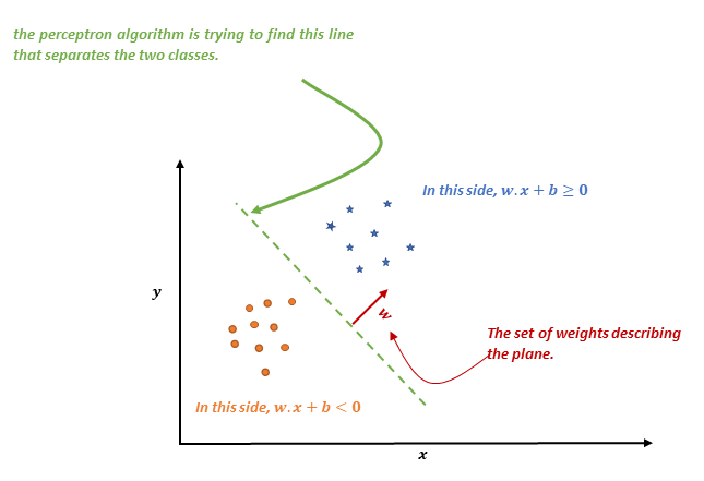
A plane can be described by a vector $w$ that is normal to the plane. Hence, when we say we want to find a separating plane we mean that we want to find the components of the vector $w$ that describe the plane.
Once the perceptron algorithm has found such hyperplane, we can classify instances based on the following rule. Note that the formula contains a bias term $b$ without this term, the hyperplane will always have to go through the origin
$$ \begin{equation} h(x)= \begin{cases} +1 & if \enspace w.x+b > 0 \newline -1 & if \enspace w.x+b < 0 \end{cases} \end{equation}$$
Here, $w.x$ is the dot product which is the sum component wise components of both vectors $\sum\limits_{i=1}^{d} w_i x_i$
The Perceptron Update Rule
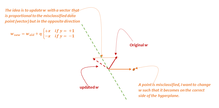
The question now is how can we find such $w$ that classifies the points correctly. A simple idea is to initialize the $w$ vector randomly and go over the points one by one. If the point is correctly classified then we do not need to do anything however, if is misclassified we need to move the hyperplane (update $w$) so that the point will eventually become correctly classified. A good choice, as shown in the next figure, is a vector that is proportional to the misclassified data point but in the opposite direction i.e. $w_{new} =w_{old}+ηyx$. The algorithm keeps iterating until $w$ converges does not change anymore.
Each iteration of the algorithm consists of a full pass over all the training examples. The algorithm terminates when in a given iteration no point was misclassified. A natural question at this point is how can we update the bias term $b$ as well. The trick is to augment our training data with all ones vector and treat the bias as another weight component (i.e. weight component of a feature whose value is alaways one).
$$ \begin{aligned} h(x) &= w.x+b \newline &= ∑{i=1}^d w_i x_i+b \newline &= ∑{i=1}^d w_i x_i+b*1 \newline &= ∑_{i=1}^{d+1} w_i x_i \end{aligned} $$
where $x_{d+1}$ always equals one and $w_{d+1}$ is the bias term
Worked Example
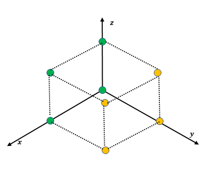
To Understand the algorithm better, let’s go through a toy example. Suppose we have the following positive and negative examples in 3D
| Positive Examples | Negative Examples |
|---|---|
| $[0 \enspace 0 \enspace 0]$ | $[0 \enspace 1 \enspace 1]$ |
| $[0 \enspace 0 \enspace 1]$ | $[0 \enspace 1 \enspace 0]$ |
| $[1 \enspace 0 \enspace 1]$ | $[1 \enspace 1 \enspace 0]$ |
| $[1 \enspace 0 \enspace 0]$ | $[1 \enspace 1 \enspace 1]$ |
Iteration 1
| Weight $[w_0 \enspace w_1 \enspace w_2 \enspace b]$ | Data $[x_0 \enspace x_1 \enspace x_2 \enspace 1]$ | ${w.x}$ | Label | Comment | New weight |
|---|---|---|---|---|---|
| $[0 \enspace 0\enspace 0\enspace 0]$ | $[0 \enspace 0 \enspace 0 \enspace 1]$ | $0 \leq 0$ | $+$ | Wrong. Add sample | $[0 \enspace 0 \enspace 0 \enspace 1]$ |
| $[0 \enspace 0 \enspace 0 \enspace 1]$ | $[0 \enspace 0 \enspace 1 \enspace 1]$ | $1 > 0$ | $+$ | OK | No Change |
| $[0 \enspace 0 \enspace 0 \enspace 1]$ | $[0 \enspace 1 \enspace 0 \enspace 1]$ | $1 > 0$ | $-$ | Wrong. Subtract sample | $[0 \enspace {-1} \enspace 0 \enspace 0]$ |
| $[0 \enspace {-1} \enspace 0 \enspace 0]$ | $[0 \enspace 1 \enspace 1 \enspace 1]$ | ${-1} < 0$ | $-$ | OK | No Change |
| $[0 \enspace {-1} \enspace 0 \enspace 0]$ | $[1 \enspace 0 \enspace 0 \enspace 1]$ | $0 \leq 0$ | $+$ | Wrong. Add sample | $[1 \enspace {-1} \enspace 0 \enspace 1]$ |
| $[1 \enspace {-1} \enspace 0 \enspace 1]$ | $[1 \enspace 0 \enspace 1 \enspace 1]$ | $2 > 0$ | $+$ | OK | No Change |
| $[1 \enspace {-1} \enspace 0 \enspace 1]$ | $[1 \enspace 1 \enspace 0 \enspace 1]$ | $1 > 0$ | $-$ | Wrong. Subtract sample | $[0 \enspace {-2} \enspace 0 \enspace 0]$ |
| $[0 \enspace {-2} \enspace 0 \enspace 0]$ | $[1 \enspace 1 \enspace 1 \enspace 1]$ | ${-2} < 0$ | $-$ | OK | No Change |
Iteration 2
| Weight $[w_0 \enspace w_1 \enspace w_2 \enspace b]$ | Data $[x_0 \enspace x_1 \enspace x_2 \enspace 1]$ | ${w.x}$ | Label | Comment | New weight |
|---|---|---|---|---|---|
| $[0 \enspace {-2}\enspace 0\enspace 0]$ | $[0 \enspace 0 \enspace 0 \enspace 1]$ | $0 \leq 0$ | $+$ | Wrong. Add sample | $[0 \enspace {-2} \enspace 0 \enspace 1]$ |
| $[0 \enspace {-2} \enspace 0 \enspace 1]$ | $[0 \enspace 0 \enspace 1 \enspace 1]$ | $1 > 0$ | $+$ | OK | No Change |
| $[0 \enspace {-2} \enspace 0 \enspace 1]$ | $[0 \enspace 1 \enspace 0 \enspace 1]$ | ${-1} < 0$ | $-$ | OK | No Change |
| $[0 \enspace {-2} \enspace 0 \enspace 1]$ | $[0 \enspace 1 \enspace 1 \enspace 1]$ | ${-1} < 0$ | $-$ | OK | No Change |
| $[0 \enspace {-2} \enspace 0 \enspace 1]$ | $[1 \enspace 0 \enspace 0 \enspace 1]$ | $1 > 0$ | $+$ | OK | No Change |
| $[0 \enspace {-2} \enspace 0 \enspace 1]$ | $[1 \enspace 0 \enspace 1 \enspace 1]$ | $1 > 0$ | $+$ | OK | No Change |
| $[0 \enspace {-2} \enspace 0 \enspace 1]$ | $[1 \enspace 1 \enspace 0 \enspace 1]$ | ${-1} < 0$ | $-$ | OK | No Change |
| $[0 \enspace {-2} \enspace 0 \enspace 1]$ | $[1 \enspace 1 \enspace 1 \enspace 1]$ | ${-1} < 0$ | $-$ | OK | No Change |
Iteration 3
| Weight $[w_0 \enspace w_1 \enspace w_2 \enspace b]$ | Data $[x_0 \enspace x_1 \enspace x_2 \enspace 1]$ | ${w.x}$ | Label | Comment | New weight |
|---|---|---|---|---|---|
| $[0 \enspace {-2}\enspace 0\enspace 1]$ | $[0 \enspace 0 \enspace 0 \enspace 1]$ | $1 > 0$ | $+$ | OK | No Change |
| $[0 \enspace {-2} \enspace 0 \enspace 1]$ | $[0 \enspace 0 \enspace 1 \enspace 1]$ | $1 > 0$ | $+$ | OK | No Change |
| $[0 \enspace {-2} \enspace 0 \enspace 1]$ | $[0 \enspace 1 \enspace 0 \enspace 1]$ | ${-1} < 0$ | $-$ | OK | No Change |
| $[0 \enspace {-2} \enspace 0 \enspace 1]$ | $[0 \enspace 1 \enspace 1 \enspace 1]$ | ${-1} < 0$ | $-$ | OK | No Change |
| $[0 \enspace {-2} \enspace 0 \enspace 1]$ | $[1 \enspace 0 \enspace 0 \enspace 1]$ | $1 > 0$ | $+$ | OK | No Change |
| $[0 \enspace {-2} \enspace 0 \enspace 1]$ | $[1 \enspace 0 \enspace 1 \enspace 1]$ | $1 > 0$ | $+$ | OK | No Change |
| $[0 \enspace {-2} \enspace 0 \enspace 1]$ | $[1 \enspace 1 \enspace 0 \enspace 1]$ | ${-1} < 0$ | $-$ | OK | No Change |
| $[0 \enspace {-2} \enspace 0 \enspace 1]$ | $[1 \enspace 1 \enspace 1 \enspace 1]$ | ${-1} < 0$ | $-$ | OK | No Change |
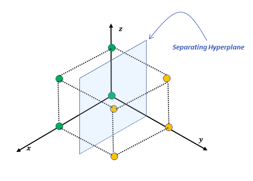
So, the hyperplane found by the perceptron algorithm can be $[0 \enspace {-2} \enspace 0 \enspace 1]$
Limitations: XOR Example
However, there is one caveat for the Perceptron algorithm. The data needs to be linearly separable otherwise, the perceptron algorithm will fail to find a solution. To illustrate this point let’s consider the case of the XOR function. The XOR function outputs a 1 if only one of the inputs is one, otherwise it outputs zero.
| Input 1 | Input 2 | Output |
|---|---|---|
| 0 | 0 | 0 |
| 0 | 1 | 1 |
| 1 | 0 | 1 |
| 1 | 1 | 0 |
We can visualize the XOR output in the 2D space as shown below. There is no line that can separate the positive from the negative points which means the data is not linearly separable.
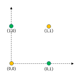
If we try to follow the same update rule specified earlier we will get stuck in an infinite loop.
Iteration 1
| Weight $[w_0 \enspace w_1 \enspace b]$ | Data $[x_0 \enspace x_1 \enspace 1]$ | ${w.x}$ | Label | Comment | New weight |
|---|---|---|---|---|---|
| $[0 \enspace 0\enspace 0]$ | $[0 \enspace 0 \enspace 1]$ | $0 \leq 0$ | $-$ | OK | No Change |
| $[0 \enspace 0\enspace 0]$ | $[0 \enspace 1 \enspace 1]$ | $0 \leq 0$ | $+$ | Wrong. Add sample | $[0 \enspace 1\enspace 1]$ |
| $[0 \enspace 1\enspace 1]$ | $[1 \enspace 1 \enspace 1]$ | $2 > 0$ | $-$ | Wrong. Subtract sample | $[{-1} \enspace 0\enspace 0]$ |
| $[{-1} \enspace 0\enspace 0]$ | $[1 \enspace 0 \enspace 1]$ | ${-1} < 0$ | $+$ | Wrong. Add sample | $[0 \enspace 0\enspace 1]$ |
Iteration 2
| Weight $[w_0 \enspace w_1 \enspace b]$ | Data $[x_0 \enspace x_1 \enspace 1]$ | ${w.x}$ | Label | Comment | New weight |
|---|---|---|---|---|---|
| $[0 \enspace 0\enspace 1]$ | $[0 \enspace 0 \enspace 1]$ | $1 > 0$ | $-$ | Wrong. Subtract sample | $[0 \enspace 0\enspace 0]$ |
| $[0 \enspace 0\enspace 0]$ | $[0 \enspace 1 \enspace 1]$ | $0 \leq 0$ | $+$ | Wrong. Add sample | $[0 \enspace 1\enspace 1]$ |
| $[0 \enspace 1\enspace 1]$ | $[1 \enspace 1 \enspace 1]$ | $2 > 0$ | $-$ | Wrong. Subtract sample | $[{-1} \enspace 0\enspace 0]$ |
| $[{-1} \enspace 0\enspace 0]$ | $[1 \enspace 0 \enspace 1]$ | ${-1} < 0$ | $+$ | Wrong. Add sample | $[0 \enspace 0\enspace 1]$ |
And we are back to the same weight that we started the seconditeration with and we become stuck in the same pattern no matter how many passes we make over the data.
Python Implementation
We can easily implement the above update rule in a couple of lines of python.
def perceptron(X, y):
    # append ones to input for bias
    X = np.hstack((X, np.ones((X.shape[0],1))))

    #limit to number of iterations to do before giving up
    max_iterations = 1000
    curr_iter = 0

    n,d = X.shape

    # initialize w to all zero vector
    w = np.zeros(d)

    while (curr_iter < max_iterations):
        mistakes = 0
        curr_iter += 1
        for i in range(n):
            yhat = -1 if np.dot(w, X[i]) <= 0 else 1
            if (yhat != y[i]):
                mistakes += 1
                w += y[i]*X[i]
        # if a pass contains no mistakes then we are done!
        if mistakes == 0:
            break

    #return the normal to the plane and bias
    return w[:-1], w[-1]
Once we found the weights using the update rule on the training data we can use them to predict new test instances by using the dot product.
def predict(x, w, b):
    yhat = np.dot(w, x) + b
    if yhat > 0:
        return 1
    else:
        return -1
Conclusion
In this post, we looked at the perceptron algorithm. We then looked at the Perceptron Update Rule and visualized some examples. We also discussed when the algorithm will succeed. i.e., when the data is linearly separable.